The Technical Guide to Additive Blending: Math, Shaders, and Advanced Effects
Beyond Simple Transparency
Picture a vibrant nebula in deep space. Think about the searing heat of an explosion. Imagine the ethereal glow of a magical spell. These powerful visual effects share something important – they all use the same technical foundation.
The secret behind these luminous, emissive visuals is a rendering technique called **additive blending**.
Here’s how it works in simple terms. Additive blending combines colors by adding the pixel values from a new object (the source) to the pixel values already on the screen (the destination). This process always makes the image brighter. It perfectly simulates adding light to a scene.
This is very different from standard alpha blending. Alpha blending simulates transparency by mixing two colors based on an alpha value.
This guide gives you a complete technical breakdown of additive blending. We will cover several key areas:
The core mathematical formula behind the effect.
How it works in the graphics pipeline and shader code.
A comparison with other essential blending modes.
Practical case studies for creating iconic visual effects.
Common pitfalls and advanced rendering considerations.

How Additive Blending Works
To truly master additive blending, you need to understand its foundational principle. It simulates adding light, not mixing paint.
A Projector Analogy
Imagine a dark room with a single white screen. You have two projectors.
One projector casts a pure red image onto the screen. The second projector casts a pure green image that partially overlaps the first.
Where only the red light hits the screen, it appears red. Where only the green light hits, it appears green. But here’s the crucial part – where both light beams overlap, the screen becomes bright yellow. This happens because red light and green light add together to create yellow light.
This physical phenomenon perfectly demonstrates additive blending in computer graphics. The core concept is simple: we are adding light sources together. This is fundamentally different from subtractive mixing, like with paints, where red and green would produce a muddy brown.
The Blending Equation
Modern graphics APIs like OpenGL, DirectX, and Vulkan use a single, powerful equation for all blending operations.
FinalColor = (SourceColor * SourceFactor) + (DestinationColor * DestinationFactor)
Let’s break down each component of this universal formula.
SourceColor is the color of the pixel from the new object we are currently trying to draw. For example, a particle of fire.
DestinationColor is the color of the pixel that is already in the frame’s color buffer. For example, the background behind the fire.
SourceFactor and DestinationFactor are configurable multipliers. These factors define the specific type of blending mode we want to use. They tell the GPU exactly how to combine the source and destination colors.
To achieve classic additive blending, we set these factors to their simplest possible values: ONE.
The SourceFactor is set to ONE. The DestinationFactor is also set to ONE.
This simplifies the general blending equation. The specific formula for additive blending becomes: FinalColor = (SourceColor * 1) + (DestinationColor * 1).
The final color is simply the source color added directly to the destination color.
Calculation Examples
The result of this addition is then “clamped.” This means any color channel value that exceeds the maximum is clipped to that maximum. The maximum is typically 1.0 in a standard pipeline, or the display’s maximum brightness. For example, a calculated color of (1.2, 0.8, 1.5) would be clamped to (1.0, 0.8, 1.0).
This clamping can lead to “white-out.” We will cover this topic in a later section.
The table below shows several additive blending calculations. Notice how black behaves as a transparent color. Adding zero has no effect.
Source Color (RGBA) | Destination Color (RGBA) | Calculation (Source + Dest) | Final Clamped Color | Visual Result |
Red (1, 0, 0, 1) | Blue (0, 0, 1, 1) | (1, 0, 1, 2) | Magenta (1, 0, 1, 1) | Colors combine |
Grey (0.5, 0.5, 0.5, 1) | Grey (0.5, 0.5, 0.5, 1) | (1, 1, 1, 2) | White (1, 1, 1, 1) | Brightness increases to max |
Black (0, 0, 0, 1) | Green (0, 1, 0, 1) | (0, 1, 0, 2) | Green (0, 1, 0, 1) | Source is invisible |
White (1, 1, 1, 1) | Any Color (r, g, b, a) | (1+r, 1+g, 1+b, 1+a) | White (1, 1, 1, 1) | Over-exposure to white |
The Alpha Channel’s Role
The alpha channel often causes confusion. In a pure ONE, ONE additive blend, the source color’s alpha value is effectively ignored during the RGB color calculation.
The “transparency” of the effect is not controlled by alpha. It’s controlled by luminance. Black pixels (0,0,0) are transparent because adding zero does not change the destination color. Brighter pixels are more opaque and contribute more light.
However, there’s a very common and useful variation of additive blending. This variant configures the blend function as (SourceFactor = SRC_ALPHA, DestinationFactor = ONE).
This is sometimes called “premultiplied alpha” blending. More colloquially, it’s called “screen” blending, though it’s not identical to Photoshop’s Screen mode. In this mode, the source color is first multiplied by its own alpha value before being added to the destination.
This allows an artist to use the alpha channel of a texture to modulate the intensity of the light being added. It provides finer control over the effect’s shape and softness.
Implementation in Shaders
Translating the theory of additive blending into practice involves two steps. You need to configure the graphics pipeline’s render state and write a shader to output the correct source color.
Configuring Render State
Blending is a state within the GPU’s output merger stage. It must be enabled and configured before you issue a draw call for an object that requires it.
The specific API calls vary. But the principle is identical across all modern graphics hardware.
In OpenGL, the setup is direct and simple. You enable blending and then set the blend function.
// Enable the blending stage glEnable(GL_BLEND); // Set the factors for additive blending glBlendFunc(GL_ONE, GL_ONE);
In Direct3D 11 or 12, this configuration is part of a larger state object. Typically a D3D11_BLEND_DESC or D3D12_BLEND_DESC struct.
Within this structure, you would set the SrcBlend and DestBlend members of the render target blend description to D3D11_BLEND_ONE or D3D12_BLEND_ONE.
Higher-level game engines abstract these API calls. In Unity’s shader language (ShaderLab), you simply add the line Blend One One within a pass definition.
In Unreal Engine, this is a material property. You would navigate to the material’s details panel and set its Blend Mode to “Additive.”
A Simple Shader Example
Once the render state is configured for additive blending, the GPU needs a source color to add. This color is the output of your object’s fragment (or pixel) shader.
Let’s look at a minimal GLSL fragment shader for a simple, textured particle. This could be a spark or a piece of an explosion.
// Simple GLSL Fragment Shader for an additive particle #version 330 core out vec4 FragColor; in vec2 TexCoords; uniform sampler2D particleTexture; uniform vec4 particleColor; void main() { // The texture often defines the shape and softness of the particle. // A grayscale texture’s R channel can represent intensity. float intensity = texture(particleTexture, TexCoords).r; // Modulate a base color by the texture’s intensity. // This becomes the SourceColor in the blend equation. FragColor = particleColor * intensity; // In a (ONE, ONE) blend, the output alpha is often irrelevant // for the color calculation, but it’s good practice to set it. FragColor.a = 1.0; }
Let’s analyze this code. The particleTexture is a 2D texture. It’s often a soft, blurry, grayscale image of a circle or “puff.”
We sample this texture using the incoming texture coordinates (TexCoords). We assume the texture’s intensity is stored in its red channel (.r).
This intensity value ranges from 0.0 (for black parts of the texture) to 1.0 (for white parts). It’s then multiplied by a uniform particleColor. This allows us to tint the particle to any color we want, like orange for fire.
The final calculated FragColor is the output of the shader. This value becomes the SourceColor that the GPU’s blending hardware will add to the DestinationColor already in the framebuffer, according to the Blend One One state we configured.
Comparing Blend Modes
To use additive blending effectively, you need to understand how it differs from other common blend modes. Choosing the right mode is essential for achieving the desired visual outcome.
Core Differences
We can summarize the primary intent of the three most common blend modes.
Additive blending adds color values. Its purpose is to simulate the emission and accumulation of light. It always brightens the scene.
Alpha blending (also called Normal or Standard blending) mixes colors based on the source’s alpha channel. Its purpose is to simulate transparency and composite layers.
Multiplicative blending multiplies color values. Its purpose is to simulate shadows, tinting, or filtering, such as looking through colored glass. It almost always darkens the scene.
Detailed Blend Comparison
A side-by-side technical comparison reveals the mathematical and practical distinctions. These guide our choice of which blend mode to use for a given task. Each mode has a distinct formula and a “transparent” color that makes it uniquely suited for certain effects.
Feature | Additive Blending | Alpha Blending (Normal) | Multiplicative Blending |
Formula | Src * 1 + Dst * 1
| Src * SrcAlpha + Dst * (1 - SrcAlpha)
| Src * Dst or Src * 0 + Dst * Src
|
Primary Use Case | Fire, magic, explosions, glows, lens flares, holograms. | Glass, smoke, water, ghost-like figures, UI overlays. | Shadows, decals (stains, bullet holes), color filtering, day/night cycles. |
Effect on Brightness | Always increases brightness (unless source is black). | Interpolates between source and destination. | Always decreases brightness (unless source is white). |
“Transparent” Color | Black (0, 0, 0) | Any color with an Alpha of 0. | White (1, 1, 1) |
Order Dependency | Order-independent. A + B is the same as B + A. | Order-dependent. Drawing a red glass in front of blue is different from blue in front of red. | Order-independent. A * B is the same as B * A. |
One of the most important but often overlooked differences is order dependency.
Additive and multiplicative blending are commutative operations. The order in which you draw objects does not change the final result. A + B is identical to B + A. This is a huge advantage for particle systems, where sorting thousands of particles by depth can be prohibitively expensive.
Standard alpha blending, however, is order-dependent. Drawing a semi-transparent red object over a blue one yields a different result than drawing the blue one over the red one. This requires transparent objects to be sorted from back to front to render correctly. This can introduce performance overhead and complexity.
Visualizing the Results
Let’s imagine a simple test case. We are drawing a soft-edged, circular red sprite onto a solid blue background.
With **additive blending**, the result would be a bright, glowing orb. The center, where red is added to blue, would be a vibrant magenta. The soft edges of the red sprite would create a smooth, glowing falloff against the blue.
With **alpha blending**, the result would look like a piece of red, semi-transparent plastic placed over the blue background. You would see a faded red circle. The blue background would be visible through it. The final color would be a mix, not a sum.
With **multiplicative blending**, the result would be a dark, purplish circle. The red sprite acts like a filter that absorbs light. Since the red sprite’s color has no blue or green components, it effectively multiplies the destination’s blue channel by a low value and the others by zero. This darkens the area significantly.
Advanced Applications
Moving from theory to practice, we can see how additive blending works behind many iconic visual effects in games and film.
Case Study: Particle Effects
Complex, dynamic effects like fire and explosions are often built from thousands of very simple elements. A particle system emits a large number of sprites. Each sprite is a simple 2D quad with a texture.
These particles are rendered with **additive blending**.
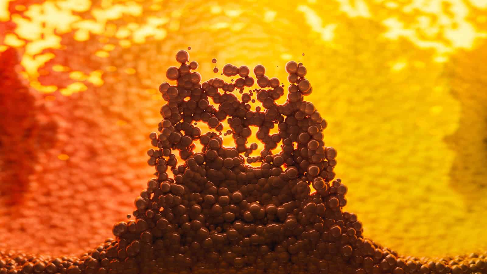
The magic happens when these particles overlap. In the core of an explosion, many bright particles are drawn on top of each other. Their color values accumulate, quickly pushing the core’s color towards bright yellow and then white. This simulates intense heat.
On the outer edges of the effect, fewer particles overlap. The colors here remain in the orange and red spectrum. This creates a natural-looking heat gradient. The use of a soft, blurry texture on each particle ensures there are no hard edges. The entire effect blends together seamlessly.
By varying the color-over-life and size-over-life of the particles, artists can create incredibly realistic and dynamic effects. For example, particles might go from yellow to red to black smoke.
Case Study: Sci-Fi Holograms
Additive blending is the perfect tool for creating the classic sci-fi holographic display. The goal is to make an object look like it is constructed from pure light.
The process involves rendering the hologram’s geometry with a material that uses additive blending. This could be a 3D model or a UI panel. This immediately gives it a luminous quality, especially against a darker scene background.
To enhance the effect, artists often use textures with fine scanlines or subtle noise patterns. These are scrolled across the model’s surface to create a sense of flickering energy.
A more advanced technique involves incorporating a Fresnel effect into the hologram’s shader. A Fresnel term calculates the angle between the surface normal and the camera’s view direction.
The shader can then be programmed to make the surface brighter at grazing angles. These are areas where the surface is almost parallel to the view direction. It becomes more transparent at direct angles. This gives the hologram a sense of volume and an energetic rim-lighting effect that greatly enhances the illusion.
Case Study: Lens Flares and Bloom
Effects that simulate camera artifacts, like lens flares and bloom, are fundamentally based on the principle of adding light.
A lens flare is created by rendering a series of textured planes (quads) aligned with the camera and a light source. These textures represent the various artifacts caused by light scattering inside a camera lens. This includes streaks, hexagonal or circular halos, and glows. Each of these elements is rendered with additive blending to combine them into a believable composite flare.
Bloom, or glow, is a post-processing effect that mimics the way very bright light bleeds into surrounding areas on a film or sensor. It’s a more generalized version of a flare.
The process typically involves several steps:
The 3D scene is rendered into an off-screen texture.
A second, smaller texture is created by running a “bright pass” filter on the first one. This extracts only the pixels above a certain brightness threshold.
This small texture of bright spots is then heavily blurred using multiple down-sampling and up-sampling passes.
Finally, this blurred “glow” texture is combined with the original scene image using **additive blending**. This adds a soft, luminous halo around all the bright objects in the scene.
Effect | Key Components | Texture Advice | Shader Tip |
Explosion | Particle System, Color-over-life, Size-over-life | Soft, radial gradient (“puff” texture) | Use texture alpha or a grayscale value to control particle shape and intensity. |
Hologram | 3D Model, Scanline overlay, Fresnel effect | Texture with fine horizontal lines and digital noise. | Implement a Fresnel term based on dot(normal, viewDir) to create bright edges. |
Lens Flare | Multiple textured planes, Parented to a light source | Various shapes: anamorphic streaks, hexagons, circles. | Animate the alpha or color of individual flare elements based on the light’s screen position. |
Limitations and Pitfalls
While powerful, additive blending is not a universal solution. Understanding its limitations and common pitfalls is key to using it professionally and avoiding visual artifacts.
The White-Out Problem
The most common issue encountered with additive blending is over-saturation. This is often called “white-out” or “blow-out.”
Because color values are always being added, it is very easy for multiple bright, additive effects to overlap. They can push the final pixel color to the maximum value of (1.0, 1.0, 1.0) in a standard low-dynamic-range (LDR) pipeline.
When this happens, the area becomes pure, flat white. All shape, texture, and color detail is lost. This can look cheap and uncontrolled, especially in effects-heavy scenes.
Advanced Solutions
The professional solution to the white-out problem lies in adopting a modern rendering pipeline.
A light-on-dark art style is a simple first step. Additive effects inherently look best when their source textures are not excessively bright. They should be rendered against a darker background, which gives the “light” room to be added without immediately hitting the ceiling.
The true technical solution is High Dynamic Range (HDR) rendering. In an HDR pipeline, the internal color buffers are not limited to a [0, 1] range. They use floating-point formats that can store much higher color values. For example, 10.0, 50.0, or more.
Additive blending is performed in this HDR space. Colors can accumulate to physically plausible energy levels without being prematurely clamped. The “white-out” still happens, but at a much higher threshold.
A final post-processing step called tonemapping is then applied. The tonemapper is a function that intelligently maps the wide range of HDR values back down to the [0, 1] range that a standard display can show. It does this in a non-linear, visually pleasing way, much like a real camera’s sensor. This preserves detail and color in both the very bright and very dark areas of the image.
For simpler pipelines without HDR, a crude solution is to manually clamp the color values in the shader. However, this is a destructive approach that can create unnatural-looking flat spots in an effect.
Finally, it’s critical to recognize when additive blending is simply the wrong tool. For simulating standard transparent materials like glass or water, alpha blending is the correct choice. For creating darkened effects like shadows or scorch marks, multiplicative blending is more effective.
Conclusion: Mastering Light
Additive blending is a fundamental technique in computer graphics. Its principle is elegant and simple: it is used for adding light, not for mixing color.
By understanding its behavior, we can create a vast array of stunning visual effects. These add energy, vibrancy, and impact to any rendered scene.
Let’s recap the key technical takeaways:
The formula is a direct addition: FinalColor = SourceColor + DestinationColor.
Black (0,0,0) acts as the “transparent” color, making it ideal for texturing effects drawn onto the scene.
It is the go-to technique for fire, glows, explosions, magic, and other emissive or energy-based effects.
Be mindful of over-saturation and use an HDR rendering pipeline with tonemapping for professional-quality results that avoid “white-out.”
Mastering the math, implementation, and artistic application of additive blending is a crucial step. Any developer or technical artist looking to elevate the quality and dynamic power of their visual effects needs this knowledge.